Gibbs-Based Information Criteria and the Over-Parameterized Regime

Based on the paper by Haobo Chen, Yuheng Bu, and Gregory W. Wornell (arXiv:2306.05583)

Motivation

Classical model selection criteria—AIC and BIC—break down in the over-parameterized regime ($p > n$), where models perfectly interpolate training data yet still generalize well (the double descent phenomenon). This occurs because:

The asymptotic normality of MLE fails,
Laplace approximation (used in BIC) becomes invalid,
There are infinitely many interpolating solutions.

To address this, the authors propose Gibbs-based AIC and BIC, derived from an information-theoretic analysis of the Gibbs algorithm. These criteria remain well-defined even when $p \gg n$.

Key Concepts

0. Introduction and Key Definitions

Before diving into the results, let us clarify the core concepts used throughout this post:

AIC (Akaike Information Criterion): A model selection criterion that approximates the expected generalization error (population risk). In its classical form:
$\mathrm{AIC} = L_E + \frac{p}{n},$
where $L_E$ is empirical risk, p is the number of model parameters, and n is the number of samples.
BIC (Bayesian Information Criterion): A criterion that approximates the log marginal likelihood of the data under a model. Classically:
$\mathrm{BIC} = L_E + \frac{p \log n}{2n}.$
Double descent: A phenomenon where test error first decreases, then increases (classical U-shaped curve), and decreases again once the model becomes over-parameterized (p > n) and can perfectly interpolate the training data.
p: Number of trainable parameters in the model (e.g., weights in the second layer of a random feature model).
SGLD (Stochastic Gradient Langevin Dynamics): A sampling algorithm that adds Gaussian noise to SGD updates to approximate samples from the Gibbs posterior.
w: model weights
n: sample size
s: samples from $(X_i, y_i)$
MALA (Metropolis-Adjusted Langevin Algorithm): A more sophisticated Markov Chain Monte Carlo method that also samples from the Gibbs posterior, but with a Metropolis-Hastings correction step for faster convergence.

In the classical regime ($p \ll n$), AIC and BIC work well. But in the over-parameterized regime ($p \gg n$), they break down—this paper proposes Gibbs-based AIC and BIC that remain valid in both settings.

1. Gibbs Algorithm

Instead of a point estimate like MLE, the Gibbs algorithm defines a posterior distribution over parameters:

\[P_{W|S}(w|s) = \frac{\pi(w) \exp(-\beta L_E(w, s))}{\mathbb{E}_\pi[\exp(-\beta L_E(W, s))]},\]

where:

$\pi(w)$ is a prior (e.g., Gaussian),
$L_E(w, s) = \frac{1}{n} \sum_{i=1}^n \ell(w, z_i)$ is empirical risk,
$\beta > 0$ is an inverse-temperature parameter.

This distribution minimizes the Information Risk:

\[\min_{P_{W|S}} \mathbb{E}[L_E(W,S)] + \frac{1}{\beta} D(P_{W|S} \| \pi \mid P_S).\]

In practice, samples from this distribution can be obtained via SGLD or MALA.

Sample-wise comparison

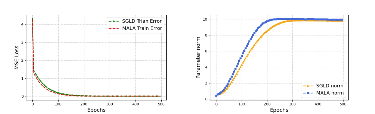
The training MSE losses of MALA and SGLD are presented on the left image, with a comparative analysis of their $L_2$ norms shown on the right image.

2. Gibbs-Based AIC

The expected generalization error of the Gibbs algorithm is exactly:

\[\mathrm{gen}(P_{W|S}, P_S) = \frac{I_{\mathrm{SKL}}(P_{W|S}, P_S)}{\beta},\]

where $I_{\mathrm{SKL}}$ is the symmetrized KL information:

\[I_{\mathrm{SKL}}(P_{W,S}) = D(P_{W,S} \| P_W \otimes P_S) + D(P_W \otimes P_S \| P_{W,S}).\]

This leads to the Gibbs-based AIC:

\[\boxed{\mathrm{AIC}^+ = L_E(\hat{w}_{\mathrm{Gibbs}}, z^n) + \frac{1}{\beta} I_{\mathrm{SKL}}(P_{W|S}, P_S)}.\]

In the classical regime ($n \to \infty$, $p$ fixed, $\beta = n$):

\[\mathrm{AIC}^+ \to L_E + \frac{p}{n},\]

recovering the standard AIC.

3. Gibbs-Based BIC

For log-loss and $\beta = n$, the negative log-marginal likelihood satisfies:

\[-\frac{1}{n} \log m(z^n) = \mathbb{E}_{P_{W|S}}[L_E(W, z^n)] + \frac{1}{n} D(P_{W|S} \| \pi).\]

This motivates two variants:

\[\begin{aligned} \mathrm{BIC}^+ &= L_E(\hat{w}_{\mathrm{Gibbs}}, z^n) + \frac{1}{n} D(P_{W|S} \| \pi), \\ \mathrm{BIC}^- &= \mathbb{E}_\pi[L_E(W, z^n)] - \frac{1}{n} D(\pi \| P_{W|S}). \end{aligned}\]

In the classical regime:

\[\mathrm{BIC}^+ \to L_E + \frac{p \log n}{2n},\]

matching traditional BIC.

Over-Parameterized Regime: Random Feature Model

The authors analyze the Random Feature (RF) model:

\[g(x) = f\left( \frac{x^\top F}{\sqrt{d}} \right) w,\]

where $F \in \mathbb{R}^{d \times p}$ has i.i.d. $\mathcal{N}(0,1)$ entries.

With a Gaussian prior $w \sim \mathcal{N}\left(0, \frac{\sigma^2}{\lambda n} I\right)$, the Gibbs posterior is Gaussian:

\[P_{W|S} \sim \mathcal{N}(\hat{w}_\lambda, \Sigma_w), \quad \hat{w}_\lambda = (\lambda n I + B^\top B)^{-1} B^\top y,\]

where $B = f(X F / \sqrt{d}) \in \mathbb{R}^{n \times p}$.

Using random matrix theory, as $n, p \to \infty$ with $r = p/n$ fixed:

\[\mathrm{BIC}^+ = L_E(\hat{w}_{\mathrm{Gibbs}}) + \underbrace{\frac{\lambda}{2\sigma^2} \|\hat{w}_\lambda\|_2^2}_{\ell_2\text{ term}} + \underbrace{\frac{1}{2} V(1/\lambda, r) - \frac{\lambda}{8} F(1/\lambda, r)}_{\text{covariance term}},\]

with

\[\begin{aligned} F(\gamma, r) &= \left( \sqrt{\gamma}(1+\sqrt{r})^2 + 1 - \sqrt{\gamma}(1-\sqrt{r})^2 + 1 \right)^2, \\ V(\gamma, r) &= r \log\left(1 + \gamma - \frac{1}{4}F(\gamma, r)\right) - \frac{\gamma}{4} F(\gamma, r) \\ &\quad + \log\left(1 + \gamma r - \frac{1}{4}F(\gamma, r)\right). \end{aligned}\]

Experimental Insights

Double Descent vs. Marginal Likelihood

AIC⁺ (proxy for generalization error) exhibits double descent.
BIC⁺ (proxy for marginal likelihood) does not — it decreases monotonically.

This reveals a fundamental mismatch: models with best generalization are not those with highest marginal likelihood.

Double descent and BIC comparison

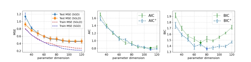
A comparison of SGD and SGLD in terms of MSE (left). Comparisons of the classical AIC with $AIC^+$ in (middle), and the classical BIC with $BIC^+$ in (right)

On this picture BIC exhibits double descent behavior while BIC+ not.

Role of the Prior ($\lambda$)

The prior variance (controlled by $\lambda$) critically shapes behavior:

Smaller $\lambda$ → flatter posterior → smaller $\ell_2$ norm → better generalization.
But BIC⁺ penalizes large $\lambda$ more heavily.

KL divergence vs generalization

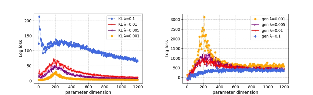
A comparison between the KL-divergence term in $BIC^+$ (left) and the generalization error term in $AIC^+$ (right) with varying λ.

Decomposition of BIC⁺ Penalty

The penalty in BIC⁺ splits into:

$\ell_2$ term: decreases with $p$,
Covariance term: captures spectral properties of $B^\top B$.

Covariance divergence term

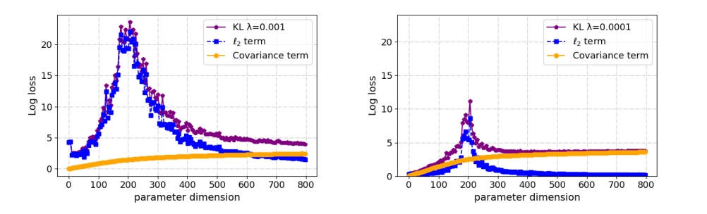
A decomposition of the terms in over-parameterized $BIC^+$ with λ = 0.001 (left), and λ = 0.0001(right).

Model Selection Performance

Classical BIC incorrectly favors moderate $p$.
Gibbs-based BIC⁺ correctly selects large $p$, aligning with low test error.

BIC comparison across criteria

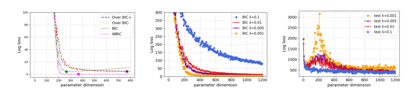
A comparison between different BICs in over-parameterized RF model when λ = 0.001 (left); A comparison between BIC+ (middle) and population risk (right) with varying λ.

Conclusion

Gibbs-based AIC/BIC provide a unified framework for model selection in both classical and over-parameterized regimes.
They remain well-defined even when MLE is non-unique.
Marginal likelihood (BIC) ≠ generalization error (AIC) in over-parameterized settings — a key insight for modern ML.
The choice of prior ($\lambda$) is not just regularization: it fundamentally alters model selection.

This work bridges information theory, Bayesian inference, and deep learning phenomena like double descent.

References

Chen, H., Bu, Y., & Wornell, G. W. (2023). Gibbs-Based Information Criteria and the Over-Parameterized Regime. arXiv:2306.05583.
Watanabe, S. (2013). A Widely Applicable Bayesian Information Criterion. JMLR.
Belkin, M., et al. (2019). Reconciling modern machine learning and the bias-variance tradeoff. PNAS.